Image segmentation algorithm

In this section image segmentation algorithm is introduced based on the clustering technique proposed in Section 4. The algorithm is based on the assumption that salient regions in an image are presented by dense clouds of points in the range domain, the feature space spanned by color coordinates. Revealed clusters of pixels are mapped to image segments, spatially continuous regions in the image.

Before describing the details of the algorithm, we comment the selection of the range domain. Since the use of the radially symmetric kernel relies on the Euclidean metric, the implemented color space should satisfy the assumption that the difference between two colors is proportional to the length of the straight line joining them. Although the proposed algorithm is not designed for any particular color space, the performance could degrade if the assumed Euclidean metric of the color space is not valid. Further discussion hereafter refers to the algorithm implementation in approximately uniform $L^*u^*v^*$ color space.

The Fast two-step histogram-based image segmentation algorithm (FHS) can be described in following steps:

1. Color space transformation
   Minimal bounding rectangle (MBR) of the input data $D=\{x_1,...,x_N\}$ in the designated color space is determined, where $x_1, ..., x_N$ are image pixels represented by their color coordinates and $N$ is the number of pixels. The computational complexity of this step is $O(N)$.
2. Domain discretization
   The range domain is partitioned into cells with side length $\sigma = h_0/\rho$, where fixed bandwidth $h_0$ and proportionality factor $\rho$ are algorithm parameters.
3. Initial density estimation
   The discrete density $\tilde{f}^D$ is acquired by counting pixels which populate each histogram cell. Proportionality constant $\lambda$ is computed as the geometric mean of $\tilde{f}^D$. The complexity of this step is $O(N)$.
4. Adaptive density estimation
   The discrete density $\hat{f}^D$ is estimated according to (15) using the Epanechnikov kernel (17):

   $$K_E(x) = \left\{ \begin{array}{ll} \frac{1}{2}c_d^{-1}(d+2)(1-\Ve... ...or } \Vert x\Vert\leq 1\\ 0 & \mbox{\ for } \Vert x\Vert>1 \end{array} \right.,$$ (17)

   
   
   where $c_d$ is equal to the volume of the $d$-dimensional hypersphere.

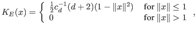
   As the influence of the Epanechnikov kernel centered at $x_i$ vanishes for $d(x,x_i) > h(x_i)$, the contribution of all samples populating the $v$-th cell with center $c_v$ is accounted for in the set of cells with center $c$ satisfying $d(c,c_v) \leq h(c_v)$. The variable bandwidth $h(x)$ is computed (8) from the initial estimate $\tilde{f}^D$. The computational complexity of this step is $O(rM)$, where $M$ is the number of populated cells and $r \propto \rho^3$.

5. Range domain clustering
   The step wise hill-climbing procedure, outlined in Section 4.2, is started from cells satisfying $\tilde{f}^D > 0$. The hill-climbing procedure partitions the input data into clusters of pixels pertaining to basins of attraction determined by strong attractors satisfying $\hat{f}^D > \varepsilon \Lambda$ and noise, where $\Lambda$ is the geometric mean of $\hat{f}^D$ and $\varepsilon$ is the algorithm parameter. The computational complexity of this step is $O(M)$.
6. Mapping range domain clusters to the spatial image domain
   Spatial constraints of image regions are recovered using the region growing procedure. The growing process is continued as long as adjacent pixels belong to the same range domain cluster. The computational complexity of this step is $O(N)$.

The region growing mapping procedure is selected to evaluate the ability of the proposed histogram-based approach to produce quality segmentations. When implemented as a part of a complex vision system, the output of the algorithm can be accommodated for a particular application and the desired input for higher level processing modules. An alternative mapping procedure (step 6) could be based on the fuzzy region growing [31], with fuzzy segments which retain uncertainty for propagation to higher level processing, where more intelligent decisions can be made. Overall complexity of the FHS algorithm is $O(3N+(r+1)M)$.

Figure 1: Normalized number of strong attractors in the range domain with respect to the relative noise level $\varepsilon$. The results are given for two values of fixed bandwidth.

[$h_0 = 8$]

[$h_0 = 12$]

The algorithm is driven by three controlling parameters: fixed bandwidth $h_0$, discretization granularity $\rho$ and relative noise level $\varepsilon$. Noise level, separating statistically important clusters from the noise and outliers, is given by (16) relatively to the geometric mean of the estimated density. In Fig. 1 number of clusters (strong attractors) in the range domain with respect to the relative noise level $\varepsilon$ is shown, normalized by the number of clusters disclosed for $\varepsilon = 1$. The results, shown for two values of $h_0$, present the average number of clusters for all images in the publicly available Berkeley Segmentation Dataset [32] collection. In both cases number of clusters for $\varepsilon = 40$ is above $99\%$ of number of clusters disclosed for $\varepsilon = 1$, suggesting low susceptibility of the algorithm with respect to this parameter. As shown in Fig. 1, the resulting number of clusters retains temporal stability starting at $\varepsilon = 9$, thus we fix relative noise level to this value.

Factor $\rho$ determines discretization granularity of the color space. This parameter prescribes the complexity of the density estimation procedure $O(rM)$, as constant $r \propto \rho^3$ directly depends on the average number of neighboring cells in the discretized domain in which kernel contribution is accounted for. We fix the discretization granularity to $\rho = 3$. This value represents a compromise between the efficiency and the quality of the provided segmentations. For greater $\rho$ space and time complexity of the algorithm rapidly grows, without prominent advances in the quality of generated segmentations.

After fixing parameters $\varepsilon$ and $\rho$, the algorithm is driven with the single parameter $h_0$ which defines the scale of observation in the range domain. The additional parameter, often used in the segmentation algorithms, can be the minimum segment size.