Subsections
Grid-based clustering with adaptive kernel density estimation
Grid-based clustering methods discretize the data domain into a finite number
of cells, forming a multidimensional grid structure on which the operations
are performed. These techniques are typically fast since they depend on the
number of cells in each dimension of the quantized space rather than the
number of actual data objects [28, p. 243].
We propose a new two-step technique for the discrete density
estimation. Firstly, initial histogram is created by counting input data
samples which populate each cell of the discretized domain. Secondly, the
sample point density estimator
(5) is applied to gain final density estimate, where
initial density estimate is used to compute variable bandwidth
(6). We will now proceed with the introduction of the
general grid-based clustering technique.
Discrete density estimation
The process of the estimation of the discrete density of the data set
 starts with domain
discretization. Bounding
starts with domain
discretization. Bounding  -dimensional hyperrectangle is determined and the
domain is partitioned into -dimensional hypercubes with side length
-dimensional hyperrectangle is determined and the
domain is partitioned into -dimensional hypercubes with side length
 . The density at some point
  is strongly influenced by a limited
set of samples near that point, thus density can be approximated with local
density function
is strongly influenced by a limited
set of samples near that point, thus density can be approximated with local
density function
 .
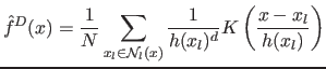
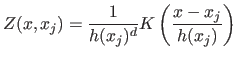
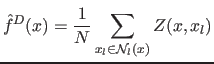
We adopt the sample point density estimation technique
(5) where each sample is assigned the variable
bandwidth (6), resulting in the adaptive local density
function:
.
We adopt the sample point density estimation technique
(5) where each sample is assigned the variable
bandwidth (6), resulting in the adaptive local density
function:
 |
(7) |
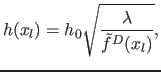
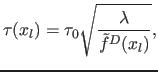
The variable bandwidth is defined by:
 |
(8) |
where
 is the initial density estimate obtained by counting data
samples which populate each cell of the multidimensional
histogram. Proportionality constant
is the initial density estimate obtained by counting data
samples which populate each cell of the multidimensional
histogram. Proportionality constant  is set to the geometric mean of
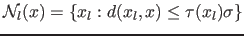
[26]. Adaptive neighborhood for each sample
is set to the geometric mean of
[26]. Adaptive neighborhood for each sample  is defined by:
 |
(9) |
where  is the variable proportionality factor. According to
(6) we define with:
is the variable proportionality factor. According to
(6) we define with:
 |
(10) |
where  is the fixed proportionality factor. The cell width is
computed from the fixed bandwidth
is the fixed proportionality factor. The cell width is
computed from the fixed bandwidth  by:
by:
 |
(11) |
where  is the discretization parameter. Setting the bandwidth to be
multiple of the cell width intuitively prescribes a set of neighboring
cells in which contribution of each sample should be accounted
for.
is the discretization parameter. Setting the bandwidth to be
multiple of the cell width intuitively prescribes a set of neighboring
cells in which contribution of each sample should be accounted
for.
The introduced PDF estimation technique requires two passes through the data
to compute the initial and the final density estimate. Efficiency of this
procedure can be increased such that it requires one pass while preserving the
accuracy. Let
 |
(12) |
be the contribution of the sample  at point . Inserting
(12) into (7) yields
at point . Inserting
(12) into (7) yields
 |
(13) |
Let  denote the spatial coordinates of the center of the
  -th histogram
cell. The contribution of all samples which populate the
-th histogram
cell. The contribution of all samples which populate the  -th cell to the
density of the -th cell is approximately
-th cell to the
density of the -th cell is approximately
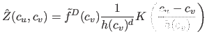 |
(14) |
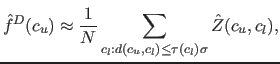
The contribution is accounted for as if all samples were
located in the center of the cell. Asset of the adaptively scaled kernel
centered at the -th cell is multiplied with the number of samples
populating that cell. By inserting
(14) into (13)
we obtain:
 |
(15) |
where
 is estimated discrete density of the -th
cell. The approximation in (14)
computes the contribution of all samples which populate a single cell in one
pass.
is estimated discrete density of the -th
cell. The approximation in (14)
computes the contribution of all samples which populate a single cell in one
pass.
The basic feature of all grid-based clustering techniques is a low
computational complexity. However, discretization unavoidably introduces error
and lowers the performance in disclosing clusters of different scales which
are often present in the real data. Some techniques attempt to solve this
problem by allowing arbitrary mesh refinement in densely populated areas
[29,30]. The resulting grid structure has complex neighboring
relations between adjacent cells, which introduces computational overhead in
the clustering procedure. Moreover, an additional pass through the data is
often required to construct the adaptive grid.
The proposed technique is based on a single resolution grid, thus a simple
hill-climbing procedure can efficiently detect modes and associated basins of
attraction. The estimator is self-tuned to the local scale variations in the
data set by using the variable bandwidth and adaptive neighbourhood. The
density estimation algorithm requires one pass through the input data and an
additional pass through populated cells, yielding computational complexity
 , where
  is cardinality of the data set,
  is the number of
populated cells and constant
is the number of
populated cells and constant  , proportional to
  , is the average
number of neighboring cells in which kernel contribution is accounted for.
, is the average
number of neighboring cells in which kernel contribution is accounted for.
Clustering and noise level
Clustering is based on determining strong density attractors and the
associated basins of attraction of the estimated discrete density. Subset of
input samples pertaining to a basin of attraction of a strong attractor is
assigned a unique cluster label. Samples pertaining to basins of attraction of
attractors with the density below noise level  are labeled as noise. Step
wise hill-climbing procedure started from populated cells (satisfying
are labeled as noise. Step
wise hill-climbing procedure started from populated cells (satisfying
 ) has two stopping criteria:
- Local maxima detected
If the density  of the detected maxima is below noise level
, all cells on the path of the hill-climbing procedure are labeled as
noise. Otherwise, a strong attractor is detected and a new label denoting
new cluster is assigned to all cells on the path of the procedure.
of the detected maxima is below noise level
, all cells on the path of the hill-climbing procedure are labeled as
noise. Otherwise, a strong attractor is detected and a new label denoting
new cluster is assigned to all cells on the path of the procedure.
- Cell with already assigned label detected
Continuation of the procedure from this point leads to an already detected
maxima. The encountered label is assigned to all cells on the path of the
hill-climbing procedure, regardless of representing noise or clustered
data.
Clustering procedure stops when all populated cells are labeled. As prior
knowledge would be required to anticipate absolute noise level, we define
relative to PDF by:
 |
(16) |
where  is the geometric mean of and
 is the
algorithm parameter. Note that value differs from the
proportionality constant , defined as the geometric mean of the
initial density estimate. The computational complexity of the hill-climbing
procedure is
is the
algorithm parameter. Note that value differs from the
proportionality constant , defined as the geometric mean of the
initial density estimate. The computational complexity of the hill-climbing
procedure is  .
.
Damir Krstinic
2011-11-04