Density based clustering

Broad category of feature space analysis techniques rely on the estimation of the probability density function (PDF) of the data set. Estimated density reveals patterns in data distribution where dense regions correspond to clusters of the data separated by regions of low density or noise. Clustering is based on determining local maxima (modes) of PDF and associated basins of attraction. The main concept is based on the density attractor notion [22].

Definition 1 (Density attractor)   A point $x^* \in \mathbb{R}^d$ is a density attractor of the probability density function $f:\mathbb{R}^d \rightarrow \mathbb{R}$ if $x^*$ is a local maximum of $f$, that is, if there exists $\epsilon>0$ such that

$$0<\mathop{d}(x, x^*) < \epsilon \Rightarrow f(x) < f(x^*),$$ (1)

where $\mathop{d}(x,x^*)$ is the distance in $\mathbb{R}^d$.

Each density attractor of PDF delineates associated basin of attraction, a set of points $x\in \mathbb{R}^d$ for which hill-climbing procedure started at $x$ converges to $x^*$. Hill-climbing procedure can be guided by a gradient of PDF [23,24] or step-wise [22].

Definition 2 (Strong density attractor)   Strong density attractor $x^*$ is density attractor satisfying

$$f(x^*) \geq \xi,$$ (2)

where $\xi$ is a noise level.

Definition 2 defines significant density attractors with regard to the uniformly distributed noise and non-specific data samples, called outliers. Due to noise and outliers, PDF can exhibit local variations with the density low compared to the modes corresponding to significant clusters. Implicitly defined number of clusters corresponds to the number of modes above noise level.

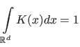
Kernel density estimation [25] is a PDF estimation method based on the concept that the density function at a continuity point can be estimated using the sample observation that falls within a region around that point.

Let $D=\{x_1,...,x_N\}$ be a set of $N$ data samples in $d$-dimensional vector space $x_i \in \mathbb{R}^d$, and $K:\mathbb{R}^d \rightarrow \mathbb{R}, K(x) \geq 0$, a radially symmetric kernel satisfying

$$\int\limits_{\mathbb{R}^d} K(x)dx = 1$$ (3)

The inherent distribution $f(x)$ of the data set $D$ at $x\in \mathbb{R}^d$ can be estimated as the average of the identically scaled kernels centered at each sample:

$$f^D(x) = \frac{1}{Nh^d} \sum_{i=1}^N K \left( \frac{x-x_i}{h} \right),$$ (4)

where bandwidth $h$ is the scaling factor.

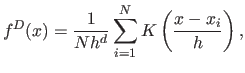
The shape of the PDF estimate is strongly influenced by the bandwidth $h$, which defines the scale of observation. Larger values of $h$ result in smoother density estimate, while for smaller values the contribution of each sample to overall density has the emphasized local character, resulting in density estimate revealing details on a finer scale. The fixed bandwidth $h$, constant across $x\in \mathbb{R}^d$, affects the estimation performance when the data exhibit local scale variations. Frequently more smoothing is needed in the tails of the distribution, while less smoothing is needed in the dense regions.

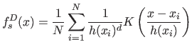
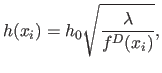
Underlying data distribution can be more accurately described using the variable bandwidth kernel. By selecting a different bandwidth $h=h(x_i)$ for each sample $x_i$, the sample point density estimator [5,26] is defined:

$$f_s^D(x) = \frac{1}{N} \sum_{i=1}^N \frac{1}{h(x_i)^d} K \left( \frac{x-x_i}{h(x_i)} \right)$$ (5)

Improvements can be obtained by setting the bandwidth $h(x_i)$ to be reciprocal to the square root [27] of the density $f^D(x_i)$

$$h(x_i) = h_0 \sqrt{\frac{\lambda}{f^D(x_i)}},$$ (6)

where $h_0$ is the fixed bandwidth and $\lambda$ is a proportionality constant. Since $f^D(x)$ is unknown density to be estimated, the practical approach [26] is to use an initial pilot estimate $\tilde{f}^D(x)$ and to take proportionality constant $\lambda$ as the geometric mean of all $\left\{\tilde{f}^D(x_i)\right\}_{i=1,...,N}$.